SingFree Directory Reference

Detailed Description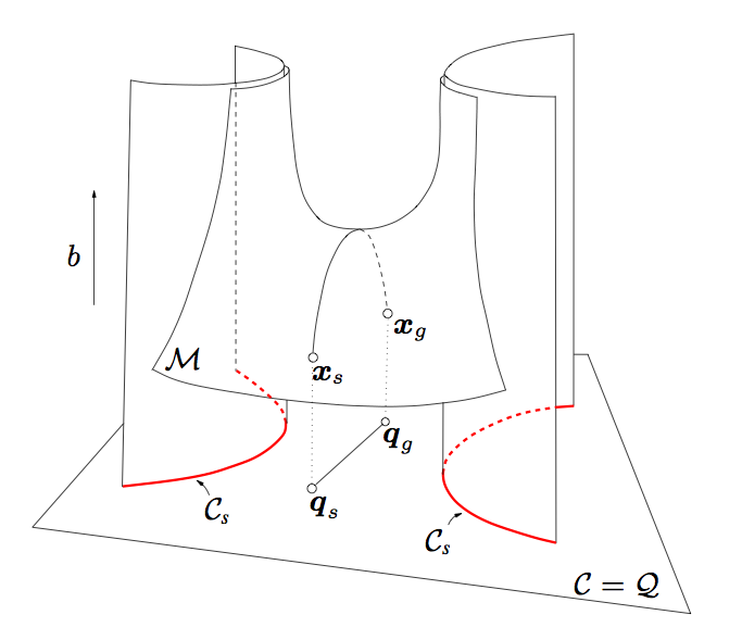

Schematic representation of the idea used to determine singularity-free paths. The singularity-free region of the configuration space is formalized as a manifold with the help of an auxiliary variable, b sending the singularities (the red curves in the plot) to infinity. Singularity-free paths are determined by navigating this new manifold.

This folder includes examples of how to define and process the appropriate equation to perform singularity-free path planning using the CuikSuite.

Note that in this case we do not define worlds, but directly cuik files. We add the singularity condition to these files, and equations to avoid reaching configurations where this condition holds. The singlarity condition is the determinant of the Jacobian. The equations to avoid the singlarity basically sends the singular configurations to the infinity by including an equation d*b=1, where d is the value of the determinant. The singularity loci can be computed by removing this equation, removing the variable b, adding an equation d=0, and using cuik. The full configuration space can be obtained witout considering the determinant constraint.

Two files are included in this folder

• simple.cuik (with the aixiliary files simple_full.cuik simple_sing.cuik)
• 3RPR.cuik (with the aixiliary files 3RPR_full.cuik 3RPR_sing.cuik)

Next, we detail the steps to find a singularity-free path and how to obtain a representation of this path:

First we obtain the singularity-free solution path (and we plot it)

• bin/cuikatlasAstar examples/SingFree/simple
• bin/cuikplotatlas examples/SingFree/simple 0 1 2
• bin/cuikplotpath examples/SingFree/simple 0 1 2

For represenation purposes, we then compute the full atlas (and we plot it)

• bin/cuikatlas examples/SingFree/simple_full
• bin/cuiktriangulateatlas examples/SingFree/simple_full 0 1 2

Moreover, to get nice final plot, we also compute the singularity loci and we plot it. Note that computing the singularity loci is significantly more expensive than computing the singularity-free path. This is the advantage of considering the singularities in implicit form during planning.

• bin/cuik examples/SingFree/simple_sing
• bin/cuikplot3d examples/SingFree/simple_sing 1 2 3 0 simple_sing.gcl

And now everything can be visualized executing

• geomview simple_sing.gcl examples/SingFree/simple_full_atlas_triang.gcl examples/SingFree/simple_atlas.gcl examples/SingFree/simple_path.gcl

After some manipulation in geomview (to change colors, etc.) you will get this plot: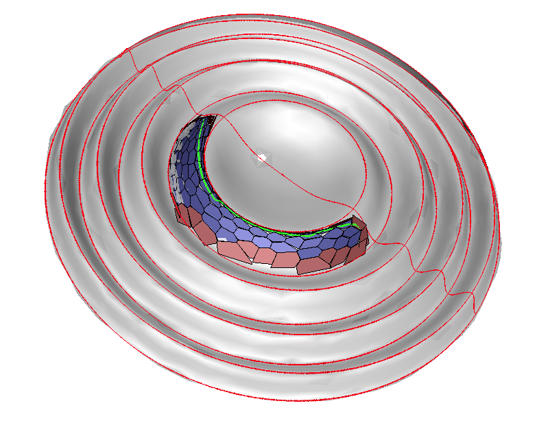

The same can be done with the 3RPR example (the only difference is that we do not triangulate the full atlas, but we plot it directly since it is much faster):

• bin/cuikatlasAstar examples/SingFree/3RPR
• bin/cuikplotatlas examples/SingFree/3RPR 0 1 2
• bin/cuikatlas examples/SingFree/3RPR_full
• bin/cuikplotatlas examples/SingFree/3RPR 0 1 2
• bin/cuikplotpath examples/SingFree/3RPR 0 1 2
• bin/cuik examples/SingFree/3RPR_sing
• bin/cuikplot3d examples/SingFree/3RPR_sing 1 2 3 0 3RPR_sing.gcl
• geomview 3RPR_sing.gcl examples/SingFree/3RPR_full_atlas.gcl examples/SingFree/3RPR_atlas.gcl examples/SingFree/3RPR_path.gcl

Again, after some manipulation in geomview you will get this figure:

For more details see our paper:

• O. Bohigas, M. E. Henderson, L. Ros, J. M. Porta,"A Singularity-free Path Planner for Closed-chain Manipulators",IEEE International Conference on Robotics and Automation, ICRA (St. Paul, USA), 2012

Files
file	3RPR_model.world [code]
	The 3RPR manipulator.